Introduction to RTK Localization Using RTKLib and the Centipede Network
Global Navigation Satellite Systems (GNSS) have revolutionized how we navigate the world. From Google Maps guiding your daily commute to precision farming equipment steering tractors with pinpoint accuracy, satellite-based positioning is everywhere. Yet, most GNSS receivers such as those in smartphones provide only a few meters of positional accuracy. For many applications, this level of precision simply isn’t enough.
Imagine a drone surveying a construction site, a robot navigating an outdoor environment, or an autonomous tractor seeding crops with millimeter precision. These tasks demand localization accuracy within a few centimeters. This is where Real-Time Kinematic (RTK) positioning comes in — a powerful technique that refines GNSS accuracy down to the centimeter level.
This article is your guide to implementing RTK-based localization using RTKLib, a powerful open-source GNSS processing tool, in conjunction with the Centipede correction data network. Whether you’re building a robotics project, doing precision mapping, or exploring GNSS for academic research, this tutorial will give you the knowledge and steps to get started.
What Is RTK Positioning?
Real-Time Kinematic (RTK) is a satellite navigation technique used to enhance the precision of position data derived from GNSS systems such as GPS, GLONASS, Galileo, and BeiDou. RTK works by using data from a fixed base station to correct the real-time position of a moving receiver, known as a rover.
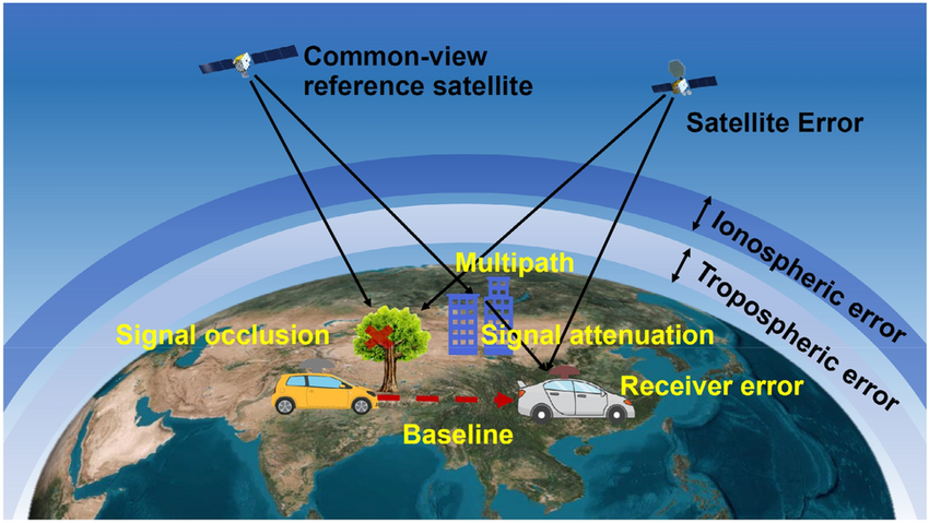
At its core, RTK is based on differential GNSS. While a standalone GNSS receiver may produce errors due to atmospheric delays, satellite clock drifts, and signal multipath, a base station at a known location can measure these errors and transmit correction data in real-time to the rover. The rover then applies these corrections to its own satellite observations, significantly improving positional accuracy, often down to just 1–2 cm.
This image shows all the common errors that are known when computing position from “classic” GNSS positioning.
RTK requires:
- A rover GNSS receiver capable of processing raw signals and corrections
- A base station (or access to one via a correction network)
- A communication link (typically over internet or radio) for real-time correction data
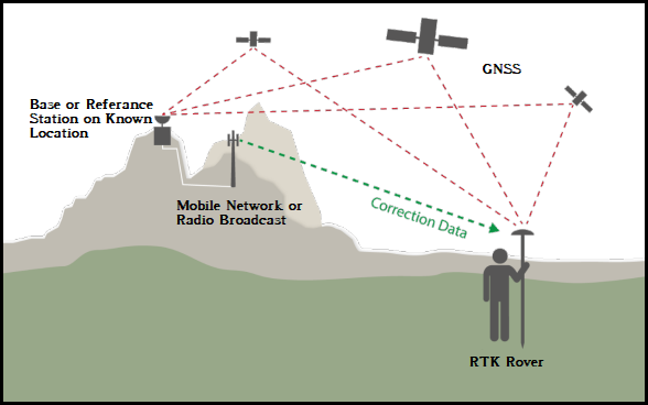
The core idea behind RTK is differential positioning. A base station with a known location calculates the error in its received GNSS signals and broadcasts these corrections in real-time to a mobile receiver, also called a rover. The rover applies these corrections to its own GNSS data to determine its precise position.
Common Use Cases for RTK
- Precision agriculture: Autonomous machinery and optimized seeding or spraying
- Land surveying: Fast, repeatable, high-accuracy positioning
- Autonomous vehicles and drones: Safe and accurate navigation
- Mapping and GIS: Collecting geospatial data with high positional fidelity
- Robotics and research: Outdoor autonomous systems needing consistent localization
More about RTK: Wikipedia - Real-time kinematic positioning
What Is the Centipede Network?
To understand how the Centipede network send data and communicate with rovers, we first need to define what is the RTCM format and the NTRIP protocol. The RTCM data format was developed by the Radio Technical Commission for Maritime Services, a non-profit international standards organization established in 1947 as a U.S. government advisory committee. In simple terms, RTCM is a data format used in the GNSS industry to communicate GNSS correction data between service providers and users. RTCM data is typically transmitted via radio signals over the internet. Once the data reaches a GNSS receiver, corrections are applied, thereby increasing the receiver’s position accuracy.
The Networked Transport of RTCM via Internet Protocol (NTRIP) is a protocol for streaming differential GPS (DGPS) corrections over the Internet for real-time kinematic positioning. NTRIP is a generic, stateless protocol based on the Hypertext Transfer Protocol HTTP/1.1 and is enhanced for GNSS data streams.
Traditionally, achieving RTK accuracy required setting up your own base station, which is very expensive and complicated for many users. Because we have no time nor money to achieve that, we will use Centipede: an open, community-driven network of GNSS base stations providing free access to RTCM correction data over the internet using the NTRIP protocol.
Interactive map of all the available bases of the Centipede network : https://docs.centipede.fr/
The Centipede project originated in Europe, particularly in France, to democratize high-precision GNSS access. It is especially appealing for DIYers, researchers, and small businesses that want professional-grade positioning accuracy without the cost of proprietary correction services.
Centipede Highlights:
- Public and free-of-charge (in many European regions)
- Uses standard protocols like RTCM and NTRIP
- Compatible with many GNSS receivers, including low-cost models like the u-blox ZED-F9P
- Easily integrates with open-source software like RTKLib
By tapping into Centipede’s base station data, your GNSS rover can perform RTK localization without needing its own base station hardware.
What Is RTKLib?
RTKLib is an open-source suite of GNSS processing tools developed by Tomoji Takasu of Tokyo University of Marine Science and Technology. It provides both real-time and post-processing capabilities, making it an invaluable toolkit for anyone working with high-precision GNSS data.
RTKLib supports:
- Real-time positioning (RTK) using correction streams
- Post-processing of GNSS logs (PPK)
- Flexible data formats: RINEX, RTCM, UBX, NMEA
- Cross-platform operation: Windows, Linux, macOS
- Integration with various GNSS hardware vendors
Key RTKLib Tools
- RTKNAVI: GUI for real-time RTK positioning
- STRSVR: Manages data streams between ports or files
- RTKRCV: Command-line version of the RTK engine
- RTKPOST: Post-processing tool for analyzing GNSS logs
RTKLib’s combination of flexibility, transparency, and cost (free!) makes it perfect for building RTK localization workflows without vendor lock-in.
For this tutorial, we will only use the C API of the RTKLib, but feel free to experiment with all the tools given by the library. The documentation can be found here : https://www.rtklib.com/prog/manual_2.4.2.pdf#page=116. This documentation is light and sometimes lacks of information, so if you want to dig deeper, you can always take a look at the source code of the library.
Official site for docs, downloads and source code: https://www.rtklib.com
Prerequisites
To get started, you will need a GNSS receiver capable of real-time correction. Unlike basic GPS chips, RTK-ready receivers support dual-frequency measurements and raw signal output. One of the cheapest options that are really great is the u-blox ZED-F9P, which is powerful and widely supported in the open-source community.
For this tutorial, you will also need a compiler such as gcc or clang in order to create your binary program using C. We will also use python in order to parse and convert some logs into csv file. Python3 and above should do the job.
Step-by-Step Tutorial: Achieve Centimeter-Level Localization
This tutorial walks you through setting up an RTK-based GNSS system using RTKLib and the Centipede network to localize a rover with centimeter-level accuracy.
1. Setup Serial Port for GNSS Receiver
Connect the GNSS receiver to your computer via USB or UART. Then:
- On Windows: Open Device Manager and look under “Ports (COM & LPT)” to find the COM port.
- On Linux/macOS: Run
ls /dev/tty*and identify ports like/dev/ttyUSB0or/dev/ttyACM0.
Use a terminal tool (TeraTerm, PuTTY, minicom) to verify NMEA data is streaming.
NMEA is a standard data format supported by all GPS manufacturers, much like ASCII is the standard for digital computer characters in the computer world. The purpose of NMEA is to give equipment users the ability to mix and match hardware and software. NMEA-formatted GPS data also makes life easier for software developers to write software for a wide variety of GPS receivers instead of having to write a custom interface for each GPS receiver.
2. Connect to Centipede Network
The Centipede network provides RTCM correction data over the internet using NTRIP (Networked Transport of RTCM via Internet Protocol).
Example NTRIP Settings:
- Caster:
caster.centipede.fr - Port:
2101 - Mountpoint: Depends on your region (e.g. for Paris we have the
IPGPbase) - Username/Password: leave blank or centipede/centipede
An example code for initializing the RTKLib streams and setup the connection with the Centipede caster can be found below:
|
|
Ensure that your rover has internet access, either via Wi-Fi or mobile tethering.
3. Receive and Process Data with RTKLib
After connecting to the Centipede caster with a precise mountpoint, our receiver will receive data from Centipede. In order to analyze this data, we need to read it from somewhere. Fortunately, the RTKLib API has the function we need : strread that takes a stream_t, a buffer and the buffer size as parameters and returns the numbers of bytes read from the stream. An example code is shown below :
|
|
We will also need to keep somewhere all the NMEA messages on the /dev/ttyUSB port in order to process and visualize it better on QGIS after that. To do so, we need to read inside a serial port. This code is generic and easily found all over the Internet so it is not detailed here. This page contains all the informations needed to do that.
NMEA have different type of messages, but the only type we are interested in is the GGA because it contains the position of the rover and the quality of the signal. The GGA messages follow this format:
<message type>, <UTC of position fix>, <latitude>, <direction of latitude>, <longitude>, <direction of longitude>, <GPS quality indicator>, <number of satellites in use>, <Horizontal Dilution of Precision (HDOP)>, <Orthometric height>, <unit of measure for orthometric height>, <geoid separation>, <unit of measure for geoid separation>, <age of differential GPS data record>, <reference station ID>, <checksum>
$GPGGA,172814.0,3723.46587704,N,12202.26957864,W,2,6,1.2,18.893,M,-25.669,M,2.0 0031*4F
The 6 fields we are interested in are:
- 0 : message type: we will only be interested in GGA messages because of their content.
- 2 : latitude: calculated latitude, in degree minute (DDMM.MMMMMMM).
- 3 : direction of latitude: north or south.
- 4 : longitude: calculated longitude, in degree minute (DDMM.MMMMMMM).
- 5 : direction of longitude: east or west.
- 6 : GPS Quality indicator: this will be useful to know the quality of the RTK corrections received.
- 0: Fix not valid
- 1: GPS fix
- 2: Differential GPS fix
- 4: RTK Fixed
- 5: RTK Float
- Note that quality 4 is the best quality of corrections (1-5cm accuracy), 5 is still great (10cm-1m accuracy) and 2 is meter level accuracy.
4. Visualize Data in QGIS
Before even installing QGIS, we will need to parse and convert the NMEA GGA data we received because these messages use the degree minute system, and we want the coordinates to be in latitude/longitude format for QGIS. We can use this simple Python script that parses the log file and creates a CSV file that will only contains 3 columns: latitude, longitude and quality of the signal.
|
|
First of all, you will need to install QGIS using this link: https://qgis.org/ and then open the software.
Steps:
-
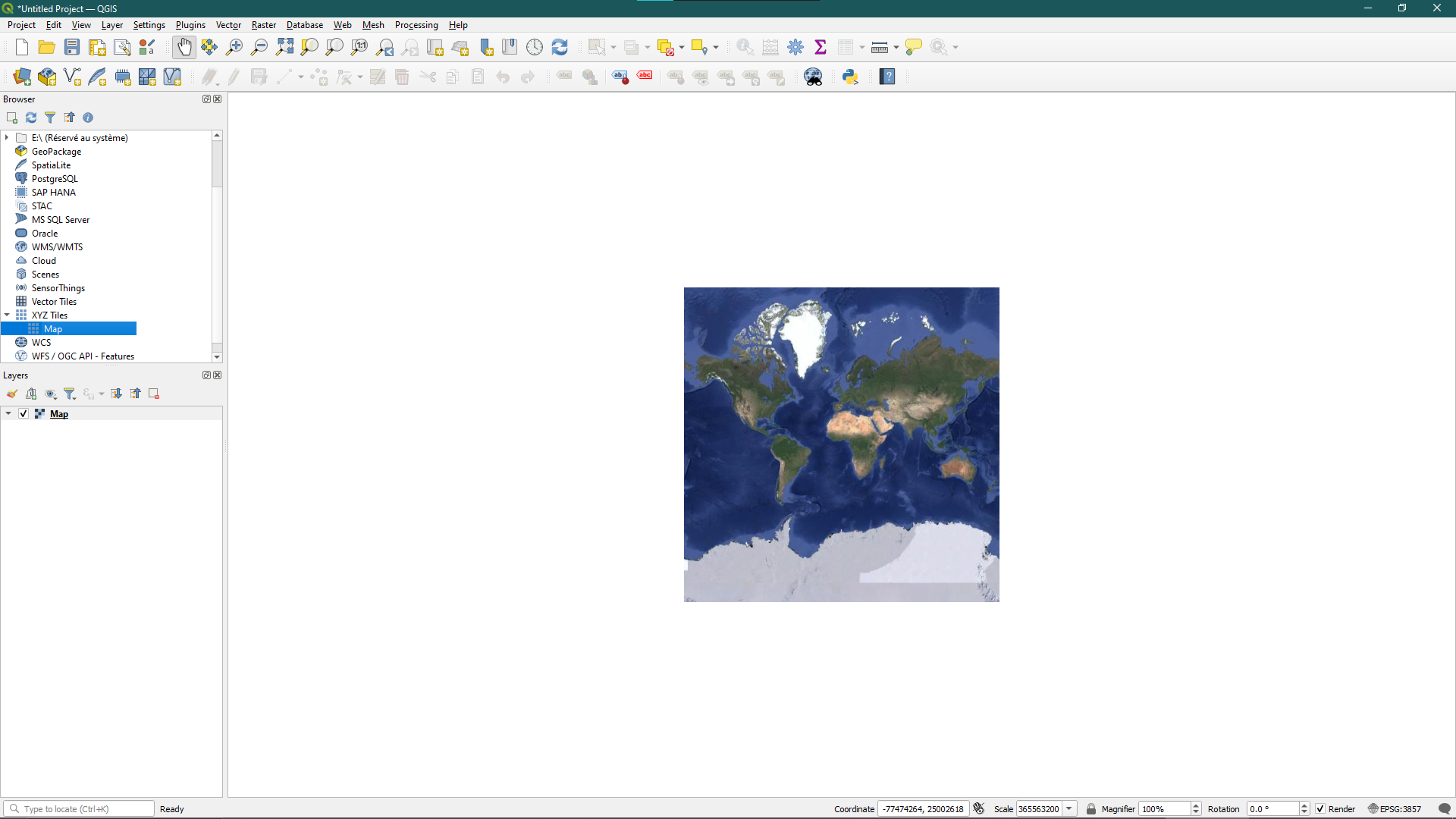
Open QGIS and click on XYZ Tiles > New Connection. In the URL field, specify this link: http://mt0.google.com/vt/lyrs=s&hl=en&x={x}&y={y}&z={z}, name the map the way you want and then click OK. Below the XYZ Tiles button there should be your map you just added, double click on it and you should have something that looks like this:
-
Load your
.csvfile generated earlier by going to Layer > Add Layer > Add Delimited Text Layer and select your file. In the Geometry Definition section, click on Point coordinates and set X field to latitude and Y field to longitude. You also need to set the Geometry CRS (Coordinate Reference System) to Default, which is WGS84 (EPSG:4326) and click on Add.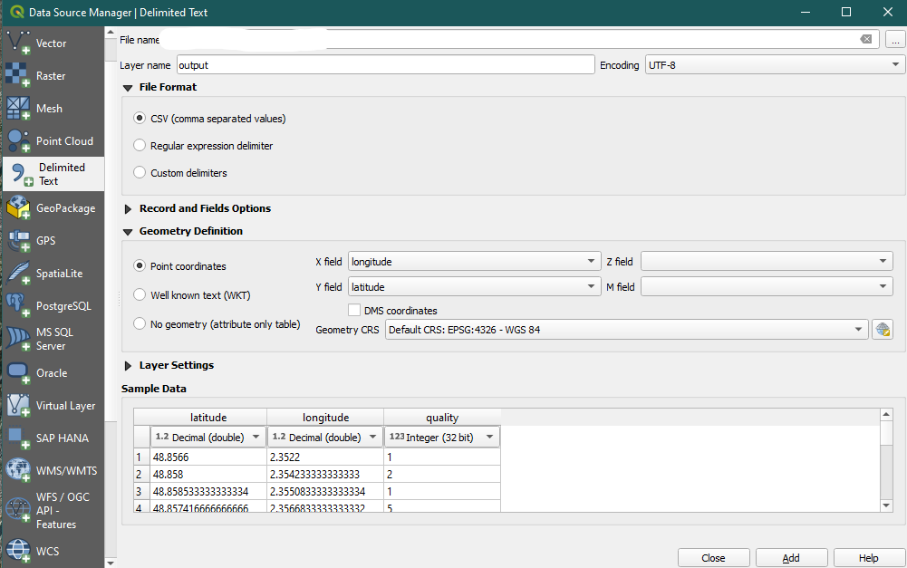
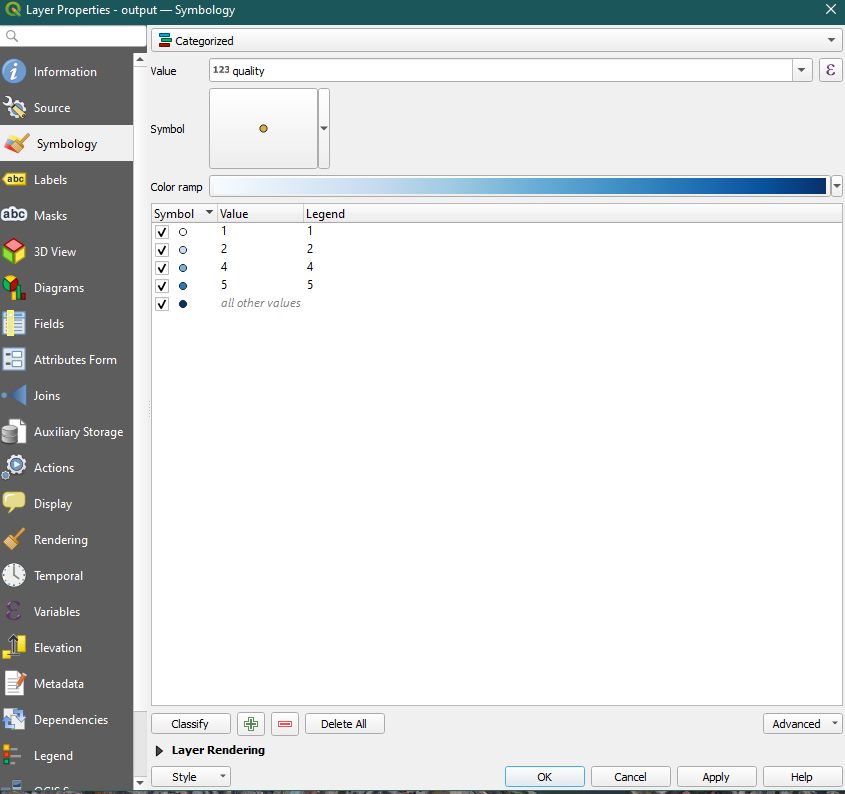
-
Double click on the left side layer you just created and go to Symbology, then select Categorized and set the value field to quality. Select a color panel and then click on classify. This should categorize the data depending on the value of the quality of the data.
In the end, using this NMEA data:
$GPGGA,120000,4851.396,N,00221.132,E,1,08,0.9,35.0,M,46.9,M,,*4A
$GPGGA,120001,4851.480,N,00221.254,E,2,10,0.8,36.1,M,46.9,M,,*45
$GPGGA,120002,4851.512,N,00221.305,E,1,09,0.7,34.9,M,46.9,M,,*4C
$GPGGA,120003,4851.445,N,00221.401,E,5,12,0.6,36.5,M,46.9,M,,*43
$GPGGA,120004,4851.388,N,00221.211,E,4,10,0.7,35.7,M,46.9,M,,*41
$GPGGA,120005,4851.477,N,00221.192,E,1,08,0.9,34.8,M,46.9,M,,*40
$GPGGA,120006,4851.365,N,00221.380,E,2,11,0.8,36.0,M,46.9,M,,*4D
$GPGGA,120007,4851.509,N,00221.230,E,1,09,1.0,35.6,M,46.9,M,,*4F
$GPGGA,120008,4851.490,N,00221.310,E,5,12,0.6,35.5,M,46.9,M,,*42
$GPGGA,120009,4851.475,N,00221.340,E,1,07,1.1,34.7,M,46.9,M,,*4B
$GPGGA,120010,4851.460,N,00221.290,E,0,00,1.2,0.0,M,0.0,M,,*6A
$GPGGA,120011,4851.425,N,00221.370,E,4,11,0.7,36.2,M,46.9,M,,*46
$GPGGA,120012,4851.410,N,00221.330,E,1,08,0.8,35.3,M,46.9,M,,*47
$GPGGA,120013,4851.388,N,00221.280,E,2,09,0.9,36.1,M,46.9,M,,*48
$GPGGA,120014,4851.360,N,00221.360,E,1,10,0.8,34.6,M,46.9,M,,*4E
$GPGGA,120015,4851.530,N,00221.260,E,1,08,0.9,35.0,M,46.9,M,,*49
$GPGGA,120016,4851.510,N,00221.390,E,5,12,0.6,35.4,M,46.9,M,,*4C
$GPGGA,120017,4851.495,N,00221.210,E,1,09,0.7,35.2,M,46.9,M,,*44
$GPGGA,120018,4851.470,N,00221.280,E,0,00,1.3,0.0,M,0.0,M,,*6C
$GPGGA,120019,4851.455,N,00221.300,E,1,08,0.8,35.1,M,46.9,M,,*4D
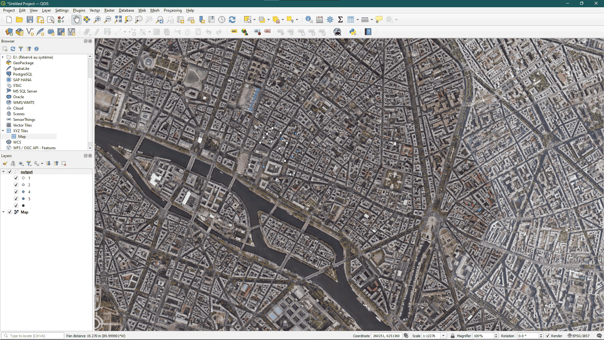
We should have a map with all the points looking like this
Code for Centipede connection
The full example code can be found here:
|
|
Conclusion
RTK positioning using RTKLib and the Centipede network is a cost-effective and open-source method for achieving centimeter-level localization. Whether you’re working in autonomous robotics, surveying, agriculture, or academic research, this setup offers flexibility and high accuracy without proprietary lock-in.
Limitations to Keep in Mind
- Satellite visibility: Buildings and trees can block signals.
- Baseline length: Accuracy degrades as distance from the reference station increases.
- Multipath effects: Reflections from surfaces can corrupt signals.
- Atmospheric conditions: Tropospheric and ionospheric delays can impact accuracy.
In optimal conditions, RTK provides centimeter-level accuracy. But for professional-grade reliability in challenging conditions, advanced techniques may be needed.
Looking Forward: Network RTK Algorithms (VRS, MAC, FKP)
While single-base RTK (like Centipede) works well within 10–20 km of a station, Network RTK expands this by using a cluster of base stations to reduce spatial decorrelation.
Main Algorithms:
- VRS (Virtual Reference Station): Interpolates corrections to simulate a virtual base station near the rover.
- MAC (Master Auxiliary Concept): Sends corrections from a master station and nearby auxiliaries.
- FKP (Flächenkorrekturparameter): Uses polynomial models to send area-based corrections.
These methods help achieve high accuracy over wider areas, reduce latency, and offer better results in dynamic environments.
Learn more: A comparison of the VRS and MAC principles for network RTK