Introduction
1.1. Motivation and Scope
3D Printing, or additive manufacturing, totally redesigned the way individuals and companies works.
For the individuals: everyone is now able to create their own items for a 10th of the original piece price. The consumer is now able to create is own objects that he couldn’t find on the marketplace too (car parts, replacement parts, …)
For companies: they are now able to prototype for twice as cheap (if not more) and twice as fast than with regular manufacturing (injection molding, CNC, …).
There is multiple 3D Printing methods (SLA: a resin is solidified by LCD screen under it, SLS: same but with lasers, …), but in this article, we will focus on the FDM (Fused Deposition Modeling) method: a thermoplastic filament is heated, melted and extruded trough the nozzle to form layers, typically flat, horizontal and stacked along a vertical axis.
This planar, layer-by-layer approach has been the best part of the 3D printing since its creation. It made the printing easy, fast, and structurally correct since it has been used for years (open-source helped a lot to get something stable).
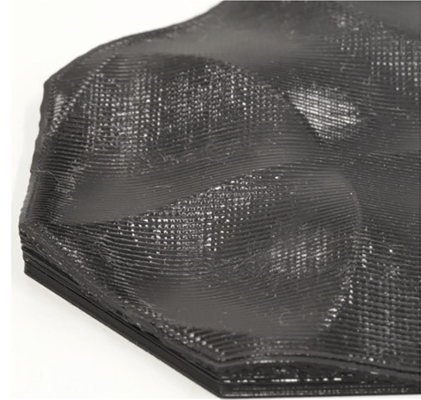
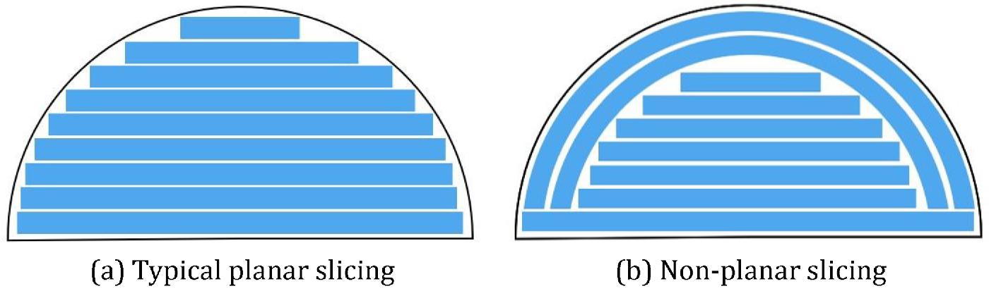
However, this slicing method, is often described as not 3D but “2.5D” printing because it stacks flat layers along a single direction (the Z-axis). These include visible layer lines on curved surfaces like that:
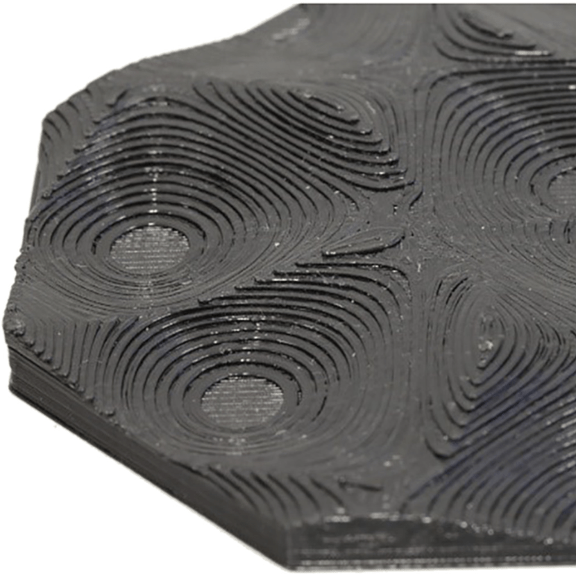
It also create mechanical weaknesses due to poor layer adhesion, and the frequent need for support structures to prop up overhanging features each of which impacts the quality, strength, and design flexibility of printed parts. The parts tends to break along the layer lines.
- Non-planar slicing enters the room -
Non-planar slicing represents a fundamental shift in additive manufacturing: instead of stacking flat, constant-thickness layers, toolpaths can now follow curved or tilted surfaces and dynamically vary layer height to conform more closely to a model’s geometry. By adapting each extrusion pass to the part’s contours, this approach creates visibly smoother surfaces, enhances interlayer adhesion for greater mechanical strength and slashes the need for support structures.
1.2. Prerequisites and Mathematical Foundations
To fully understand the transition from planar to non-planar slicing, a basic understanding of 3D printing workflows and some mathematical concepts is helpful.
The main challenge of 3D Printing is translating digital model to physical form. The digital model is an “STL” file (STereo-Lithography) which is central to this process, it represents the object as a collection of triangles.
Each triangle is defined by three vertices (points in 3D space, denoted as $x$, $y$, $z$ coordinates) and a normal vector, which indicates the triangle’s orientation, pointing outward from the object’s surface.
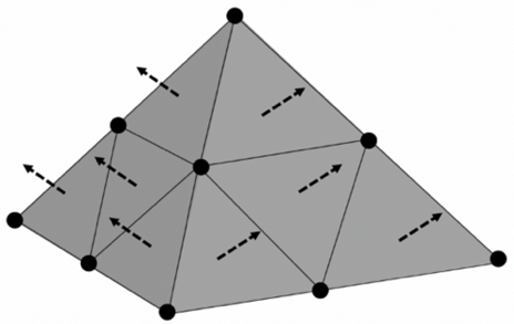
For a triangle with vertices $\mathbf{p}_1 = (x_1, y_1, z_1)$, $\mathbf{p}_2 = (x_2, y_2, z_2)$, and $\mathbf{p}_3 = (x_3, y_3, z_3)$, the normal vector $\mathbf{n}$ is calculated using the cross product of two edges:
$$\mathbf{n} = (\mathbf{p}_2 - \mathbf{p}_1) \times (\mathbf{p}_3 - \mathbf{p}_1)$$Where the components of $\mathbf{n} = (n_x, n_y, n_z)$ are:
$$n_x = (y_2 - y_1)(z_3 - z_1) - (z_2 - z_1)(y_3 - y_1)$$ $$n_y = (z_2 - z_1)(x_3 - x_1) - (x_2 - x_1)(z_3 - z_1)$$ $$n_z = (x_2 - x_1)(y_3 - y_1) - (y_2 - y_1)(x_3 - x_1)$$In planar slicing, the process involves intersecting this triangular mesh with a series of parallel planes, typically spaced evenly along the Z-axis (typically, every 0.2 mm). For a plane at height $Z = z_i$, the slicer finds where this plane cuts through each triangle, producing line segments that form a closed 2D contour for that layer. Mathematically, if a triangle’s vertices have Z-coordinates $z_1$, $z_2$, and $z_3$, and $z_{\min}$ < $z_i$ < $z_{\max}$ (where $z_{\min}$ and $z_{\max}$ are the triangle’s lowest and highest Z values), an intersection occurs. The intersection points are computed using linear interpolation along the triangle’s edges. For an edge from $\mathbf{p}_1 = (x_1, y_1, z_1)$ to $\mathbf{p}_2 = (x_2, y_2, z_2)$, the intersection at $z_i$ has coordinates:
$$x = x_1 + \frac{(z_i - z_1)(x_2 - x_1)}{z_2 - z_1}$$ $$y = y_1 + \frac{(z_i - z_1)(y_2 - y_1)}{z_2 - z_1}$$ $$z = z_i$$These calculations are repeated across all triangles for each slicing plane, forming the basis of traditional FDM printing. Non-planar slicing builds on this foundation but introduces more complex surfaces curved or tilted requiring advanced geometric and algorithmic techniques, which we’ll explore later in this article.
Conventional Planar Slicing
2.1. Overview of FDM 3D Printing
FDM is the most accessible and widely used 3D printing technology.
In FDM, a spool of thermoplastic filament such as PLA (based on corn), ABS (car plastic) or PET (plastic bottles) is fed into a heated extruder which melts the filament and deposits it onto a plate, following the GCode file (we’ll discuss about it later). This process of layering is sequential: the printer completes a layer, adjust the Z-height by raising the nozzle and begins the next layer until the object is complete.
The workflow starts with a 3D model, typically designed in CAD software like Fusion 360, which is exported as STL file. This file, as noted earlier, represents the model as a mesh of triangles.
The slicer software (Simplify3D, PrusaSlicer, BambuStudio …) takes this STL file and dissects it into horizontal slices. Each slice corresponds to a fixed Z-height, determined by the user-specified layer thickness (commonly 0.2 mm).
The slicer calculates the intersections of these planes with the STL mesh (as seen in part 1.2), producing 2D contours that outline where the filament should be deposited.
These contours are then converted into toolpaths (see 2.2).
These paths are saved in G-code file: a language originally developed for CNC machining but adapted for 3D printing.
A typical command might look like G1 X50 Y50 Z0.2 F1200 E1.5, instructing the
printer to move to position (50, 50, 0.2) at a speed of 1200 mm/min while
extruding 1.5 mm of filament. The “G1” denotes a linear move with extrusion,
while “X,” “Y,” and “Z” specify coordinates, “F” sets the feed rate, and “E”
controls extrusion volume. This granular control allows precise replication of
the digital model in physical form.
2.2. Slicer Toolpath Generation (Layering, Infill, Supports)
Once the STL file is sliced, the slicer generates toolpaths to guide the printer’s nozzle. This process involves several steps, each criticals:
-
Contour Extraction: For each layers, the slicer intersects the slicing plane with the STL mesh’s triangles. These segments are connected head-to-tail to form closed loops representing the layer’s outer and inner boundaries.
-
Perimeter Generation: The slicer offsets these contours inward by the width of the filament extrusion (0.4mm) to create perimeters or shells.
-
Infill Generation: Inside the perimeters, the slicer fills the layer with an infill pattern to provide internal structure. Infill density ranging from 0% (hollow) to 100% (solid).
-
Support Structures: For overhangs (walls that extend beyond the layer below at angles steeper than about 45°), the slicer generates temporary support structures, like scaffolds. They are easy to remove after the object is printed.
-
Toolpath Optimization: The slicer optimizes the nozzle’s path to minimize travel moves (non-extruding movements) and improve efficiency. This might involve reordering perimeter and infill sequences or adjusting speeds and extrusion rates.
The resulting toolpaths are translated into G-code, specifying every move and extrusion.
Here is an example of a sliced STL: 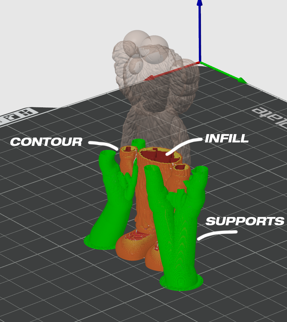
2.3. Limitations of Planar Layers
Despite its strengths, planar slicing has notable drawbacks that limit its effectiveness:
-
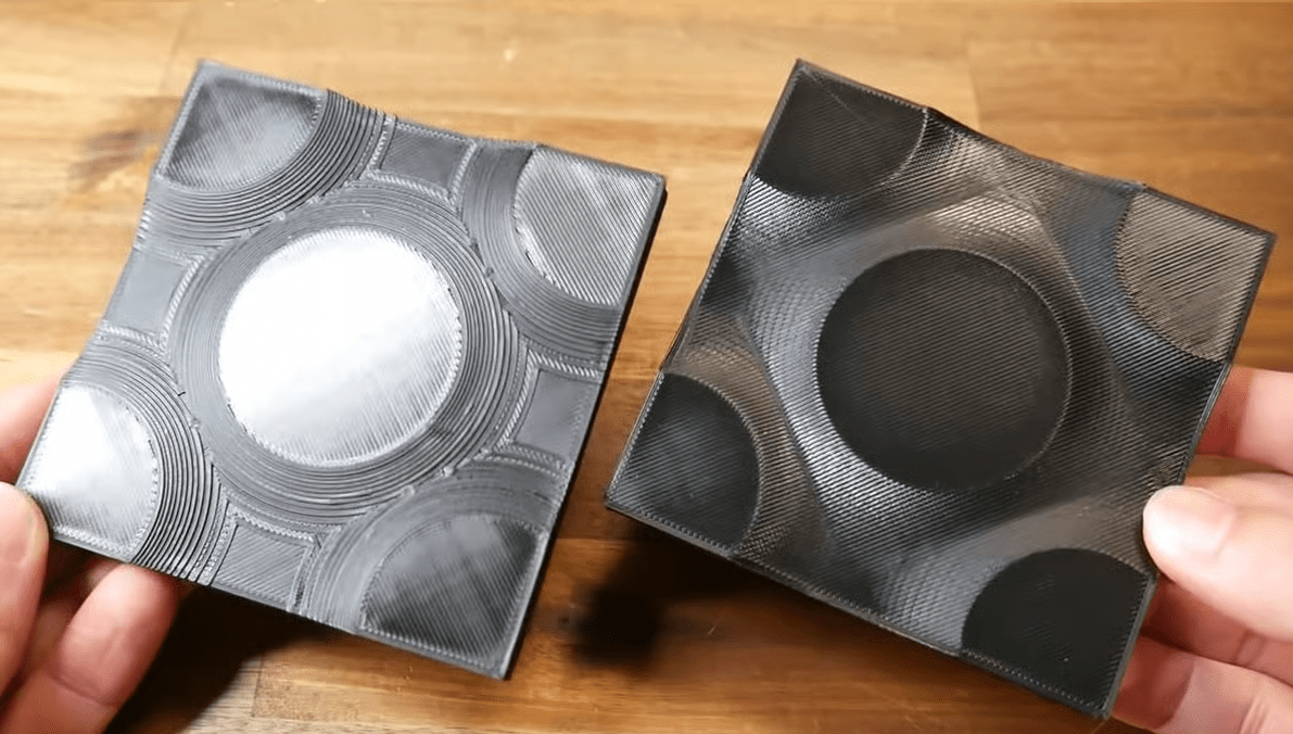
Staircase Effect: The most visible issue is the “staircase effect,” where flat layers approximate curved or slanted surfaces with stepped edges. On a curved surface, such as a sphere, each layer creates a small ledge, resulting in visible lines and a rough texture. This is especially pronounced on shallow slopes (low angles relative to the horizontal), where steps are more noticeable. Mathematically, if a surface slopes at an angle $\theta$ from the horizontal, the step width is proportional to the layer height $h$ divided by $\cos(\theta)$. For small $\theta$, $\cos(\theta)$ approaches 1, making steps subtle, but as $\theta$ decreases, steps widen, degrading surface quality.
-
Mechanical Weaknesses: These steps aren’t just cosmetic. The abrupt transitions between layers can weaken inter-layer adhesion, creating stress concentrations where cracks may form under load. Parts are often anisotropic (stronger in the XY plane than along the Z-axis) because filament bonds less effectively between stacked layers than within a single layer’s continuous roads.
-
Support Dependency: Overhangs beyond 45° require supports, as filament cannot bridge large gaps without a base. Supports increase material use, extend print time, and leave surface marks upon removal. For complex geometries this dependency restricts design freedom and adds post-processing effort.
-
Time vs. Quality Trade-off: Reducing layer height (e.g., from 0.2 mm to 0.05 mm) smooths the staircase effect but increases the number of layers, lengthening print time significantly. For a 10 cm tall object, a 0.2 mm layer height requires 500 layers, while 0.05 mm requires 2000, quadrupling the duration.
These limitations highlight the need for a new approach, setting the stage for non-planar slicing to overcome these challenges and enhance 3D printing’s capabilities.
Non-Planar Slicing Concepts
3.1. Curved and Variable-Z Toolpaths
Non-planar slicing departs from the flat-layer norm by allowing layers to curve or tilt, aligning more closely with an object’s natural shape. In traditional FDM, each layer is a planar slice at a constant Z-height, but non-planar slicing introduces variable-Z toolpaths where the Z-coordinate changes within a layer.
Imagine printing a dome: instead of stacking flat rings that approximate its curve, the printer could deposit filament along a continuous, upward-curving path, forming a smooth, bowl-like layer that matches the dome’s contour. This approach, often termed Curved-Layer FDM (CLFDM), reduces the staircase effect by following the model’s surface geometry more naturally.
Variable-Z toolpaths can take several forms. In a fully non-planar print, every layer might be a curved surface, sculpted to fit the object’s topology. Alternatively, hybrid methods combine planar and non-planar layers: a model’s base might use flat layers for stability, while upper surfaces transition to curved layers for smoothness. For instance, a 2018 study by Ahlers demonstrated printing a part with planar lower sections and a single curved top layer, achieving a polished finish without the time cost of thin planar layers across the entire object. Another strategy, multi-directional slicing, divides the model into sub-volumes, each sliced along a different axis. A concave feature might be printed with layers tilting inward, while another region remains horizontal, resulting in a composite of non-planar orientations.
These toolpaths require the printer to move in X, Y, and Z simultaneously,
rather than fixing Z during a layer. A G-code snippet for a curved path might
look like G1 X10 Y10 Z0.2 E0.1 followed by G1 X11 Y11 Z0.25 E0.15,
incrementally raising Z as the nozzle traces the curve. This flexibility
enhances surface quality and opens new design possibilities, though it demands
more from both software and hardware.
3.2. Algorithmic Differences: Planar vs. Non-Planar
The shift to non-planar slicing introduces significant algorithmic complexity. Planar slicing is straightforward: for each Z-height $z_i$, the slicer intersects the STL mesh with a plane $Z = z_i$, computes 2D contours, and generates toolpaths using established 2D geometry algorithms (e.g., polygon offsetting for perimeters, grid patterns for infill). The process is repetitive and computationally efficient, often optimized with data structures like binary trees to filter triangles by Z-range, reducing checks from $O(N \cdot L)$ (where $N$ is the number of triangles and $L$ is the number of layers) to near $O(N \log N)$.
Non-planar slicing, however, requires defining layers as curved or tilted surfaces, not just planes. One approach approximates the model’s surface with a parametric function (say, a polynomial or spline) and intersects this with the mesh. For a surface $Z = f(X, Y)$, the slicer must solve for intersections with each triangle, a task more akin to ray-tracing than simple plane cuts. This increases computational load, as the intersection points no longer lie in a single plane and may require iterative methods to refine. Another method, used in multi-directional slicing, segments the model into sub-volumes based on features (e.g., concave loops), assigns each a local slicing direction, and applies planar slicing within that orientation. The resulting layers are non-planar globally, as directions vary across the object.
Infill generation becomes trickier on curved surfaces. Planar infill relies on 2D patterns projected onto a flat layer, but non-planar infill must adapt to 3D curvature, potentially requiring 3D grid structures or projections that account for surface slope. Collision avoidance adds further complexity: the slicer must model the nozzle’s geometry and ensure it doesn’t strike protruding parts of the print during a curved move. This often involves limiting curvature steepness or simulating the print process to detect clashes.
G-code generation also differs. Planar G-code uses discrete Z-steps between layers, but non-planar G-code embeds Z-variation within moves, demanding precise coordination of X, Y, Z, and extrusion (E) to maintain filament consistency across changing heights. These algorithmic shifts make non-planar slicing a richer, more demanding problem, ripe for computational innovation.
3.3. Hardware Constraints and Printer Modifications
Standard FDM printers, with their 3-axis Cartesian or delta designs, are optimized for planar slicing. The nozzle, fixed vertically, deposits filament downward onto a flat layer, stepping up in Z between layers. Non-planar slicing pushes these machines beyond their design limits. A steep curve within a layer risks the nozzle colliding with the print, as the fixed orientation can’t adjust to surface angles. For gentle curves, a 3-axis printer can cope if the slicer limits Z-variation to avoid clearance issues, but steep overhangs or complex tilts exceed its capabilities.
Hardware modifications unlock non-planar potential. The RotBot, a modified Prusa i3, adds a fourth axis: a nozzle tilted at 45° that rotates around the Z-axis. This allows it to approach overhangs from the side, printing up to 90° without supports by leveraging its conical deposition path.
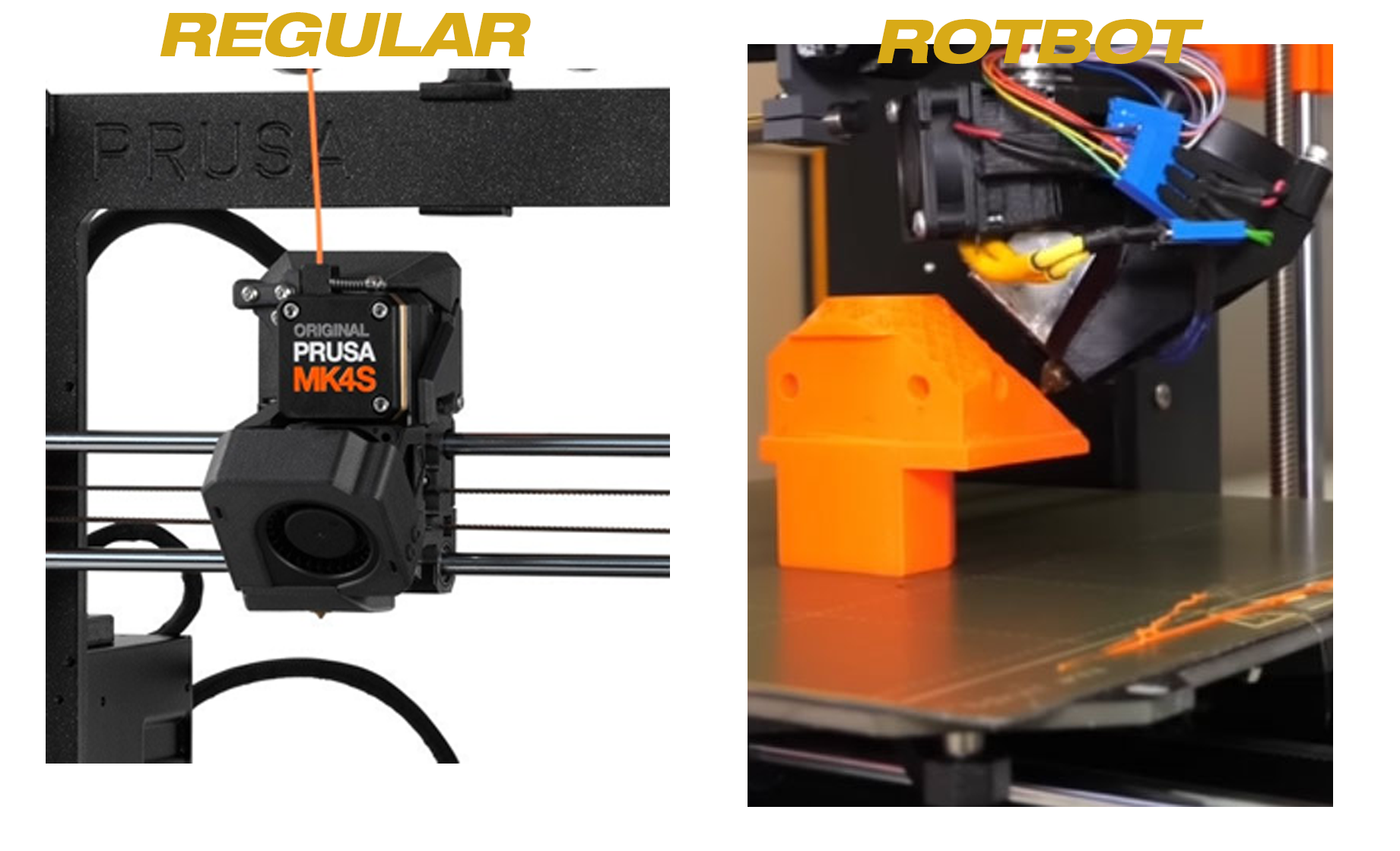
The setup requires a custom toolhead (with a slip-ring for rotation), a modified hotend, and an upgraded controller to manage the extra motor. More advanced systems, like 6-axis robotic arms, offer full orientational freedom, enabling the nozzle to remain normal to any surface: an approach explored by Roullier (2023) for composite printing. These robots, however, are costly and complex, requiring custom software pipelines (e.g., RoboDK) to translate slicing data into robotic instructions.
Even with modified hardware, challenges persist. Multi-axis motion can slow printing due to additional motor coordination, and positional accuracy may suffer from mechanical play in extra axes. Extrusion dynamics also change: filament deposited at angles may sag under gravity, necessitating enhanced cooling or material adjustments. These constraints highlight the interplay between software innovation and hardware evolution in realizing non-planar printing’s full potential.
Advantages of Non-Planar Printing
4.1. Surface Quality Improvements
Non-planar slicing dramatically enhances surface quality by eliminating the staircase effect. Curved layers follow the model’s contours, depositing filament along natural slopes rather than approximating them with flat steps. A dome printed with curved layers emerges smooth and glossy, free of the visible ridges that mar planar prints, especially on low-angle surfaces. Maissen (2024) found that fully non-planar prints reduced roughness significantly, offering near-molded finishes directly from the printer. This reduces post-processing needs (sanding or chemical smoothing). For aesthetic applications (e.g., art pieces) or functional ones (e.g., aerodynamic surfaces), this improvement is a game-changer.
4.2. Enhanced Mechanical Properties
Beyond aesthetics, non-planar layers improve mechanical performance. The staircase effect in planar prints creates weak points at layer boundaries, reducing Z-axis strength due to poor adhesion. Curved layers, especially when printed normal to the surface, enhance bonding by maximizing contact area and alignment between filament roads. This reduces anisotropy, making parts more uniformly strong. In applications like curved structural components, aligning layers with load paths can boost durability, a concept akin to fiber alignment in composites. Research suggests these properties could extend to fiber-reinforced prints, amplifying strength further.
4.3. Reduced Support Structures
Non-planar slicing minimizes support needs by enabling self-supporting geometries. A tilted or curved layer can bridge overhangs naturally, as seen in RotBot’s ability to print 90° features by approaching from the side. This saves material, shortens print time, and eliminates support removal marks, enhancing underside quality.
State of the Art and Research
5.1. Key Publications and Their Approaches
Over the past decade, researchers have steadily extended the flat‐layer paradigm of 3D printing into non‐planar realms, aiming to eliminate the “staircase” effect and boost surface fidelity. Early work by Schurig in 2015 laid the conceptual groundwork by comparing straightforward slicing methods with optimized sweep‐plane techniques to highlight the limitations of planar cuts and inspire truly curved layer strategies
Building on this foundation, in 2024 was demonstrated how conventional toolpath software like PrusaSlicer can be retrofitted for curved‐layer fused deposition modeling, significantly reducing surface roughness by warping the G‐code to conform to part geometry
In 2023, Roullier introduced a six‐axis robot slicing framework that computes normals on meshed layers, enabling multi‐directional deposition paths that follow surface contours rather than a single build plane
Shortly before, Ahlers proposed a hybrid slicing approach that interleaves minimal curved sections with traditional planar layers to optimize build speed and surface quality, demonstrating that selective curvature can balance accuracy and efficiency
5.2. Existing Software and Plugins (e.g., RotBotSlicer)
Tools like RotBotSlicer transform planar G-code into conical paths for 4-axis printing, while CurviSlicer offers a research framework for 3-axis curved slicing. PrusaSlicer modifications and Slic3r’s non-planar branch demonstrate community-driven progress, though they remain experimental.
5.3. Comparative Analysis of Current Methods
Hybrid methods balance simplicity and quality, multi-directional slicing excels for complex geometries, and full non-planar approaches maximize smoothness but demand more computation. Each suits different use cases, from hobbyist tweaks to industrial precision.
Challenges and Future Directions
6.1. Computational and Algorithmic Hurdles
Non-planar slicing’s complexity (curved surface computation, 3D infill, collision checks) requires robust algorithms and higher processing power, pushing research into optimization and real-time solutions.
6.2. Integration within Existing Slicer Ecosystems
Open-source slicers (PrusaSlicer) are adaptable, but proprietary ones (BambuLab) resist change, awaiting proven success from DIY efforts. Plugins and post-processors offer workarounds, but full integration lags.
6.3. Emerging Printer Hardware Trends
Multi-axis printers (e.g., RotBot, robotic arms) and adaptive features (variable extrusion) are emerging, promising broader non-planar adoption as costs decrease.
6.4. Outlook for the Next 2–3 Years
Expect refined algorithms, mainstream slicer support, and affordable multi-axis hardware, driven by community and industry collaboration, transitioning non-planar slicing from niche to norm.
Conclusion
Non-planar slicing heralds a dynamic future for 3D printing, overcoming planar limitations with smoother, stronger, and more efficient prints. As challenges are met, it will redefine additive manufacturing’s potential, blending software ingenuity with hardware innovation.
Bibliography
Scientific
- Schurig F. (2015). Slicing Algorithms for 3D-Printing. Student thesis, Universität München. From https://blog.hk-fs.de/wp-content/uploads/2015/08/Paper_Fabian_Schurig_3D_Printing.pdf
- Maissen S., Zürcher S., Wüthrich M. (2024). Adaptation of Conventional Toolpath-Generation Software for Use in Curved-Layer Fused Deposition Modeling https://doi.org/10.3390/jmmp8060270
- Roullier L. (2023). Non-planar slicing and Normal-to-Surface path programming https://www.ensta-bretagne.fr/jaulin/rapport2023_roullier.pdf
- Ahlers D., Wasserfall F., Hendrich N., Zhang J. (2018). 3D Printing of Nonplanar Layers for Smooth Surface Generation https://doi.org/10.1109/COASE.2019.8843116
- Zhang T., Fang G., Huang Y., Dutta N., Lefebvre S., Kilic Z. M., Wang C. C. L. (2019). CurviSlicer: Warping S3-Slicer: A General Slicing Framework for Multi-Axis 3D Printing http://dx.doi.org/10.1145/3550454.3555516
Open-source Projects & Implementations
- RotBotSlicer. Nonplanar G-code generation via geometry mapping and inverse slicing. GitHub repository: https://github.com/RotBotSlicer/Nonplanar_Slicing
- CurviSlicer. Research project for curved-layer printing on standard 3-axis FDM printers. GitHub repository: https://github.com/mfx-inria/curvislicer
Demonstrations & Media
- Non-Planar 3D Printing Demonstration. YouTube video. https://www.youtube.com/watch?v=izlbj_I1kg8
- Ultra-smooth 3D printing: non-planar ironing on all 3D printers. JanTec Engineering, YouTube. https://www.youtube.com/watch?v=VwKHgLqRezk&t=201s