Introduction

Have you ever played a video game and asked yourself: How does the game make props, characters, and objects move together in a realistic way?

Well, video game programmers use a wide variety of techniques to create movement on the screen. Ranging from directly moving pixels to simulating complex virtual worlds governed by a set of rules that can produce emergent behavior from the player’s actions.

One of the key components in a game engine responsible for describing these rules and how objects interact is called the physics engine.

Today, we’ll explore how to create a very simple set of rules and make objects interact with each other to produce motion. In other words, we’re going to simulate physics.

Physics simulation

First we need to do a proper definition of what is a physics engine. Today we will make a real time physics engine (i.e. video game physics engine) and not high precision physics engine (i.e. science simulation engine). The major differences are:

• We have to compute everything in less than 16 ms in theory (frame budget for 60 fps) and less than 5ms in practice (we can’t use the whole frame budget only for physics!)
• While this is not without consequences, we CAN miss frames and still continue the simulation

That makes our physics engine a Discrete entity based soft real time simulation engine. Let’s break that statement down

• Discrete: Unfortunately, computers cannot compute or store infinite data. So we need to transform the continuous physical rules of our world into a discrete virtual simulation. In practice, this means computing the state of the simulation at regular intervals called steps
• Entity based: Our simulation models the interactions between characters, props, or object called entities. This differs from an event-based simulation, which reacts to events triggered by actors instead of continuously modeling behavior.
• Soft real time: Real-time means the simulation must run quickly, ideally within 5–10ms per frame. Soft means it’s okay to occasionally miss a step if needed. Contrary to hard real-time systems, like a rocket’s flight computer, where skipping a step could mean mission failure..
• Simulation engine: We are computing the result of a defined mathematical model

Back to high school physics

Now, the only thing missing to start building our own physics engine is the mathematical model we want to simulate. And that’s exactly what we are going to define.

The scope of our simulation

For this little experiment, we will define a simplistic physics model. Our world will be a big black circle acting like a cage for our entities. This black circle is a static body and will not be affected by anything during the simulation. On the other hand, our entities, smaller white circles, are dynamic bodies subjected to three forces and constraints:

• The force of gravity pointing toward negative y (down) at g Newtons
• The distance constraint preventing entities from going beyond our cage
• The collision constraint preventing our entities from overlapping each other

Now that we have defined a world, an entity, and a set of rules, we have the scope of our simulation, and we can start working on transforming this into computable equations.

Newton’s second law

If we take only gravity and forget about constraints for a second, we can very easily create an equation from Newton’s second law. Remember, you did it in physics in high school.

We can transform Newton’s second law a bit to get this equation:

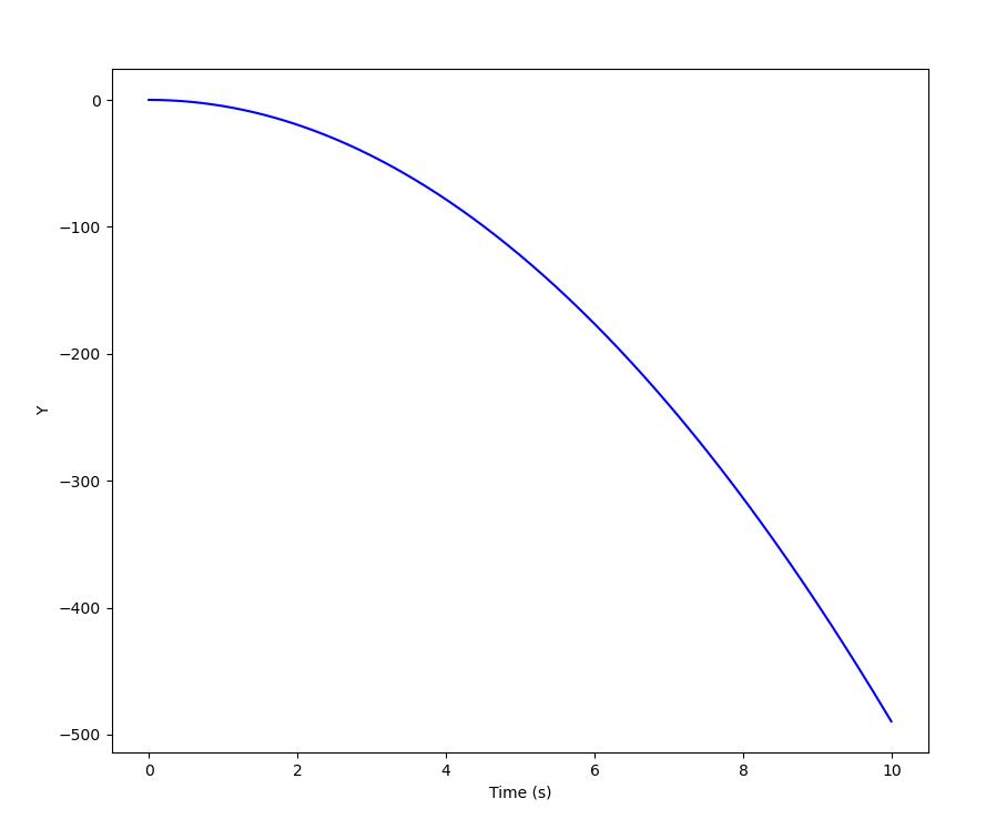
If we integrate this equation twice and suppose the initial conditions (y(t = 0) = 0 and v(t = 0) = v_0), we get the equation of motion of our object as a function of time.

We can plot that and see y falling quickly to negative infinity: that’s simply our object falling down indefinitely.

Okay, so we can just add the constraints, use the same method, and code that object_position = f(t), right? … Right?

Let’s try and apply Newton’s second law again, but this time with the constraints back in. Our constraints are defined as being 0 most of the time and something when a specific criterion is met. In our case, the criterion depends on the object’s position, so we can define our constraints as a function that takes the object’s position as a parameter.

Unfortunately, things are not so easy. To integrate an equation, we need every component of it to be integrable. Mathematical functions have many integrability criteria, but for this article, we only look at one: functions need to be continuous to be integrable. g is constant, so it is continuous (thus integrable) by definition. However, our constraints are not. For example, our distance constraint can be defined like this:

So we cannot integrate this equation like we did above. However, we have a second-degree differential equation, so maybe we could solve it directly. Unfortunately, again, the constraints are not linear, and solving non-linear differential equations analytically is impossible. Thankfully, more powerful tools exist to solve this issue.

From continuous to discrete

There are several ways to compute the result of a differential equation. Today, we will briefly look at a simple method you probably already know: the Euler method and a better one for our purposes: Verlet integration.

The simple method: Euler integration

I wont dive too deep in the mathematical theory but we can quickly find out where does it come from. Basically a second order differential equation is defined like this (remember the application of Newton’s second law above!):

To get approximate values of f(t) and f''(t), we can do two first-order Taylor expansions, giving us this system of equations:

We can rewrite the second one like this:

Now, we can just define two sequences y and z holding the values of f' and f:

Then, we can write a very simple algorithm to compute the values of the two sequences. Here is a Rust version of the Euler method:

 1
 2
 3
 4
 5
 6
 7
 8
 9
10
11
12
13
14
15
16
17

def order2Euler<F>(tf: f32, h: f32, func: F) -> (Vec<f32>, Vec<f32>)
where F -> Fn(f32, f32, f32) -> f32 {
    let mut y = 0;
    let mut z = 0;
    let mut t = 0
    let mut tt = vec![t];
    let mut tz = vec![z];
    while t < tf {
        t += h;
        y += h * z;
        z += h * func(z, y, t);
        tt.push(t);
        tz.push(z);
    }

    (tt, tz)
}

The more stable method: Verlet integration

The Euler method is good and simple to implement. It’s also not that expensive to compute (except if you want t_f = 100000 and h = 0.0001). However, the approximate value is computed using a first-order Taylor expansion. This imprecision can easily create stability issues in our simulation.

To solve this issue, we can use a mathematical trick to improve stability — at the cost of… nothing!

Verlet integration works basically the same way as Euler integration; however, it uses a Taylor expansion one degree higher than Euler’s, computing a more precise approximate value. Verlet integration works by computing the value one step before and one step after the current one and adding the two equations together, giving us this equation:

This mathematical trick makes the first and third derivatives cancel out, allowing us to completely ignore them. By manipulating this equation, we can make it easier to write as code:

By the definition of velocity, we get our final Verlet integration equation:

Building it in Rust

Now that we understand the theory, we can actually implement it in practice. And you will see that if you understood the previous part, the actual code is far from being complex.

Prerequisite

To build this basic physics engine, you need to have a basic knowledge of the Rust programming language, even though I will describe every tricky line of code. While this is not strictly necessary to implement this project (you can just plot the result of the equations), it’s far better if we can actually see our entities moving on the screen in real time. For this purpose, I used a custom OpenGL 4.5 renderer and GLFW to handle window creation. I also used a very simple shader to draw the shape of our entity.

Implement a Verlet solver

To implement a physics engine solver, we first need to define our object struct. This struct is very simple: we need to store the current position, the position at the last frame (to compute velocity), and the acceleration at this frame. In this object, we define the fn update_position(&mut self, dt: f32) method that actually does the Verlet computation.

 1
 2
 3
 4
 5
 6
 7
 8
 9
10
11
12
13
14
15
16
17
18
19
20
21
22
23
24
25
26

pub struct VerletObject {
    /* Skipping some rendering related fields */
    pub current_position: Vec2,
    old_position: Vec2,
    acceleration: Vec2,
}

impl VerletObject {
    pub fn new() -> Self {
        /* Initialize object */
    }
    pub fn update_position(&mut self, dt: f32) {

        let velocity: Vec2 = self.current_position - self.old_position;

        self.old_position = self.current_position;

        // This is the verlet equation we saw earlier
        self.current_position = self.current_position + velocity + self.acceleration * dt * dt;

        self.acceleration = Vec2::zero();
    }
    pub fn accelerate(&mut self, acc: Vec2) {
        self.acceleration += acc;
    }
}

After this, we can define the solver. This object will be used to modify each object’s attributes according to the forces and constraints applied to them. To do that, we will define a fn update(&self, objs: Vec<VerletObject>, dt: f32) method that runs every frame to update all of the objects.

As you can see, the update method takes a dt parameter. In the physics context, this value comes from the derivative and is defined as tending to 0. However, it is still simply the time difference between the last step and the current one, so we can define it as such: the time difference between now and the last frame. For example, if you run the program with vsync activated on a 60Hz screen, dt should always be very close to 16 ms.

 1
 2
 3
 4
 5
 6
 7
 8
 9
10
11
12
13
14
15
16
17
18
19
20
21
22
23
24

pub struct VerletSolver {
    gravity: Vec2,
    background_radius: f32,
    ball_radius: f32,
    sub_step: u32,
}

impl VerletSolver {
    pub fn new(grav: Vec2, background_radius: f32, ball_radius: f32, sub_step: u32) -> Self {
        Self {
            gravity: grav,
            background_radius,
            ball_radius,
            sub_step,
        }
    }
    pub fn update(&self, objs: &mut [VerletObject], dt: f32) {
        for obj in objs.iter_mut() {
            /* Perform physics computation */
        }
        self.update_position(objs, sub_dt);
    }
}

To finish our setup, we can use these two objects in the entry point of our program like this:

 1
 2
 3
 4
 5
 6
 7
 8
 9
10
11
12
13
14
15
16
17
18
19
20
21
22
23

fn main() {
    /* Renderer setup */

    let ball_radius = 0.5;
    let background_radius = 2.5;

    let mut objects = Vec::new();

    objects.push(VerletObject::new(&mut renderer));

    // Define gravity as a vector pointing downward at 9.81 m/s²
        let verlet_solver = VerletSolver::new(Vec2::new(0.0, -9.81), background_radius, ball_radius);

    let mut dt = Instant::now();

    while !window.should_close() {
        // Compute dt as the time difference between this frame and the last one.
        verlet_solver.update(&mut objects, (Instant::now() - dt).as_sec_f32());
        dt = Instant::now();

        /* Render objects */
    }
}

Gravity

After this setup is done, we can start adding features to the Verlet solver’s update method. First, we will add gravity to the mix. To do this, we simply accelerate all of our objects by the amount of VerletSolver::gravity.

 1
 2
 3
 4
 5
 6
 7
 8
 9
10
11
12
13
14
15

impl VerletSolver {
    ...

    pub fn apply_gravity(&self, obj: &mut VerletObject) {
        obj.accelerate(self.gravity);
    }

    pub fn update(&self, obj: &mut Vec<VerletObject>, dt: f32) {
        for i in 0..obj.len() {
            /* Run physic update */
            self.apply_gravity(&mut obj[i])
        }
        self.update_position(obj, dt);
    }
}

Now we can see the ball falling into the void toward negative infinity on the y-axis. It would be nice if it had a ground to bounce off, right?

Constraints

This “ground” is exactly the next step in our plan. As we saw earlier, we want our objects to be constrained inside a bigger circle. This constraint can be defined very easily: if the distance between the object and the center of the circle is greater than a certain value, we “push back” the object inside the circle. Very simple, right?

What’s great about this is that the Verlet equation takes all the bouncing and dynamics into account without us doing anything!

 1
 2
 3
 4
 5
 6
 7
 8
 9
10
11
12
13
14
15
16
17
18
19
20
21
22

impl VerletSolver {
    ...

    pub fn apply_constraint(&self, obj: &mut VerletObject) {
        let to_obj: Vec2 = obj.current_position;
        let dist = to_obj.mag();
        if dist > (self.background_radius - self.ball_radius) {
            let n = to_obj / dist;
            obj.current_position = n * (self.background_radius - self.ball_radius);
        }
    }

    pub fn update(&self, obj: &mut Vec<VerletObject>, dt: f32) {
        for i in 0..obj.len() {
            /* Run physic update */
            self.apply_gravity(&mut obj[i])
            self.apply_constraint(&mut obj[i])
        }
        self.update_position(obj, dt);
    }
}

Collision

To complete the scope we defined earlier, we need to add one more feature: collision between the objects. This one is a little more complicated because we need to compute the collision between every ball every frame, which is quite compute-intensive.

There are a lot of different algorithms, but for the sake of simplicity, we will implement a “brute force” version of collision detection. Every frame, for every object, we loop over every other object to find out if they are colliding (i.e., close enough) with the current object. This algorithm is very simple to implement but has a complexity of O(n²), which is far from ideal.

 1
 2
 3
 4
 5
 6
 7
 8
 9
10
11
12
13
14
15
16
17
18
19
20
21
22
23
24
25
26
27
28

impl VerletSolver {

    pub fn solve_collision(&self, obj_list: &mut [VerletObject]) {
        let size = obj_list.len();
        for x in 0..size {
            for y in x + 1..size {
                let collision_axis = obj_list[x].current_position - obj_list[y].current_position;
                let dist = collision_axis.mag();
                if dist < (self.ball_radius * 2.0) {
                    let n = collision_axis / dist;
                    let delta = (self.ball_radius * 2.0) - dist;
                    obj_list[x].current_position += 0.2 * delta * n;
                    obj_list[y].current_position -= 0.2 * delta * n;
                }
            }
        }
    }

    pub fn update(&self, obj: &mut Vec<VerletObject>, dt: f32) {
        self.solve_collision(obj);
        for i in 0..obj.len() {
            /* Run physic update */
            self.apply_gravity(&mut obj[i])
            self.apply_constraint(&mut obj[i])
        }
        self.update_position(obj, dt);
    }
}

As you can see, the collisions are far from perfect — they have this sort of “gooey” effect and are not very stable (the simulation can even start to diverge at some point!). We will see a very simple trick to solve this in the next part.

Increase stability

There are many possibilities to increase the stability of a simulation. As we saw earlier, the Verlet integration is already more stable than the Euler method (try it for yourself; you will see that it’s easier for the simulation to diverge with Euler), and there are methods that are even more stable.

Here, we want to stick with Verlet integration, so we need to find a trick to improve stability with this model. We can ask ourselves: what causes the instability? When we derived the Euler and Verlet integration equations, we saw that we only computed approximate values using Taylor expansions. This is what causes the instability we are not computing precise values.

There are two ways to get more precise values when using Taylor expansions:

• Increasing the order of the expansion so that the big O term contains a higher order and thus fewer terms are ignored. This is what we did to go from the Euler method to Verlet integration. However, if we cannot use a trick to cancel parts of the expansion, it can get very expensive.
• Taylor expansions are calculated for \( h \to 0 \). If we use smaller values for \( h \), we can increase precision.

We will use the second method. However, we saw that our value for \( h \) (dt in our program) is tied to the frame rate (which itself is bad, but we can overlook this for now). We could try to increase the frame rate (disabling VSync, for example), and that would definitely work. However, we cannot always increase the frame rate or disable VSync. To achieve the same effect, we will compute substeps inside the Verlet solver. To reflect this, we can make a very simple modification to our program:

 1
 2
 3
 4
 5
 6
 7
 8
 9
10
11
12
13
14
15
16
17
18
19
20
21
22
23
24
25
26
27
28
29
30
31
32
33
34
35
36
37
38
39
40
41
42
43

// verlet_solver.rs

pub struct VerletSolver {
    gravity: Vec2,
    sub_step: u32,
}

impl VerletSolver {
    pub fn new(grav: Vec2, background_radius: f32, ball_radius: f32, sub_step: u32) -> Self {
        Self {
            gravity: grav,
            background_radius,
            ball_radius,
            sub_step,
        }
    }

pub fn update(&self, objs: &mut [VerletObject], dt: f32) {
    let sub_dt = dt / self.sub_step as f32;

    for _ in 0..self.sub_step {
        self.solve_collision(objs);
        for obj in objs.iter_mut() {
            self.apply_gravity(obj);
            self.apply_constraint(obj);
        }
        self.update_position(objs, sub_dt);
    }
}

...

}

// main.rs
fn main() {
    ...
    
    let verlet_solver = VerletSolver::new(Vec2::new(0.0, -9.81), 2);
    
    ...
}

Now we can try to run it with 2 substeps:

It’s already better but not perfect. Let’s try with 6 substeps:

Nice, now we got something good. However, we have to be careful because each substep increases the compute time of the simulation, and with the O(n²) collision algorithm, it can get out of hand rather quickly.

Conclusion

To summarize, in this article, we saw how to make a physics engine from physics theory to turning these physics equations into computable problems, and finally into a proper implementation in Rust. However, the solution presented in this article is far from perfect, and there is plenty of room for optimization. The easiest and biggest factor we can improve here is our poor choice of collision detection algorithm. By using more advanced techniques such as space partitioning (e.g., octrees in 2D), we can reduce the compute time of the entire physics loop significantly and thus simulate very complex worlds.

Bibliography

• https://en.wikipedia.org/wiki/Equations_of_motion
• https://pauvre.org/~ccharign/IPT1A/09Euler/coursEuler.pdf
• https://en.wikipedia.org/wiki/Verlet_integration
• https://www.youtube.com/watch?v=lS_qeBy3aQI